Note
Go to the end to download the full example code
3. MLP
import os
import numpy as np
import pandas as pd
import matplotlib.pyplot as plt
plt.rcParams["font.family"] = "Times New Roman"

import seaborn as sns

from ai4water.models import MLP
from ai4water.utils import edf_plot
from ai4water.functional import Model
from ai4water.utils.utils import dateandtime_now
from ai4water.utils.utils import get_version_info
from ai4water.postprocessing import LossCurve, ProcessPredictions

from easy_mpl import plot, regplot, ridge, circular_bar_plot

from SeqMetrics import RegressionMetrics

from utils import evaluate_model, get_dataset, make_data

get_version_info()
{'python': '3.7.17 (default, Feb 1 2024, 16:37:31) \n[GCC 11.4.0]', 'os': 'posix', 'ai4water': '1.06', 'xgboost': '1.6.2', 'easy_mpl': '0.21.4', 'SeqMetrics': '1.3.4', 'tensorflow': '2.6.0', 'keras.api._v2.keras': '2.6.0', 'numpy': '1.19.5', 'pandas': '1.3.5', 'matplotlib': '3.4.3', 'h5py': '3.1.0', 'sklearn': '1.0.2', 'skopt': '0.9.0', 'seaborn': '0.12.1'}
dataset ,  _, _ = get_dataset(encoding="ohe")
X_train, y_train = dataset.training_data()
X_test, y_test = dataset.test_data()
original_data, _, _ = make_data()
***** Training *****
input_x shape:  (1059, 74)
target shape:  (1059, 1)
***** Test *****
input_x shape:  (455, 74)
target shape:  (455, 1)
There are total 12 input features used in this study, which are listed below.
Two of them are categorical features i.e. Adsorbent and Dye. Categorical
features have encoded using One-Hot encoder.
print(original_data.columns[:-1])
Index(['Adsorption Time (min)', 'Pyrolysis Temperature',
       'Pyrolysis Time (min)', 'Initial Concentration', 'Solution pH',
       'Adsorbent Loading', 'Volume (L)', 'Adsorption Temperature',
       'Surface Area', 'Pore Volume', 'Adsorbent', 'Dye'],
      dtype='object')
While there is one target, which is listed below
print(original_data.columns[-1])
Adsorption
path = os.path.join(os.getcwd(),'results',f'mlp_{dateandtime_now()}')
os.makedirs(path)

model = Model(
    model=MLP(units=99, num_layers=4,
              activation='relu'),
    lr=0.006440897421063212,
    input_features=dataset.input_features,
    output_features=dataset.output_features,
    epochs=600, batch_size=48,
    verbosity=0,
    prefix=path,
)
dot plot of model could not be plotted due to ('You must install pydot (`pip install pydot`) and install graphviz (see instructions at https://graphviz.gitlab.io/download/) ', 'for plot_model/model_to_dot to work.')
h = model.fit(X_train,y_train,
          validation_data=(X_test, y_test))
Training data
train_p = model.predict(x=X_train,)
argument test is deprecated and will be removed in future. Please
use 'predict_on_test_data' method instead.
evaluate_model(y_train, train_p)
mse 1923.80338105791
rmse 43.86118307863925
r2 0.9910363648744203
r2_score 0.9898076826340152
divide by zero encountered in true_divide
mape inf
mae 19.610070735640512
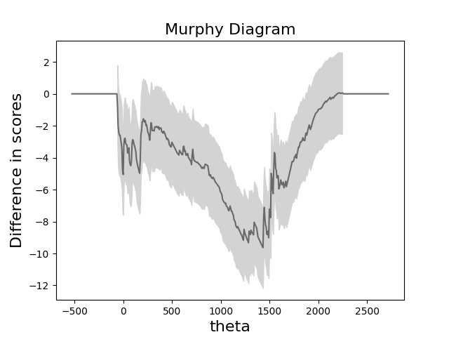
pp = ProcessPredictions(mode='regression', forecast_len=1,
                   path=path)
pp.murphy_plot(y_train,train_p, prefix="train", where=path, inputs=X_train)
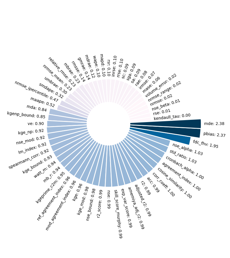
metrics = RegressionMetrics(y_train, train_p)
errors = metrics.calculate_all()

for err in ['kl_sym']:
    errors.pop(err)

n_errors = {}
for k,v in errors.items():
    if 0.<v<5.0:
        n_errors[k] = v

ax = circular_bar_plot(n_errors, sort=True, show=False, figsize=(8,9))
plt.tight_layout()
plt.show()
divide by zero encountered in log10
invalid value encountered in log10
invalid value encountered in log
divide by zero encountered in true_divide
invalid value encountered in multiply
divide by zero encountered in true_divide
invalid value encountered in log1p
divide by zero encountered in true_divide
invalid value encountered in log1p
divide by zero encountered in log
invalid value encountered in log
invalid value encountered in subtract
divide by zero encountered in true_divide
axes = regplot(pd.DataFrame(y_train), pd.DataFrame(train_p),
        marker_size=60,
        marker_color='snow',
        line_style='--',
        line_color='indigo',
        line_kws=dict(linewidth=3.0),
        scatter_kws=dict(linewidths=1.1, edgecolors=np.array([56, 86, 199])/255,
                         marker="8",
                         alpha=0.7
                         ),
        show=False
        )
axes.annotate(f'$R^2$: {round(RegressionMetrics(y_train,train_p).r2(), 3)}',
              xy=(0.3, 0.95),
              xycoords='axes fraction',
              horizontalalignment='right', verticalalignment='top',
              fontsize=16)
plt.show()

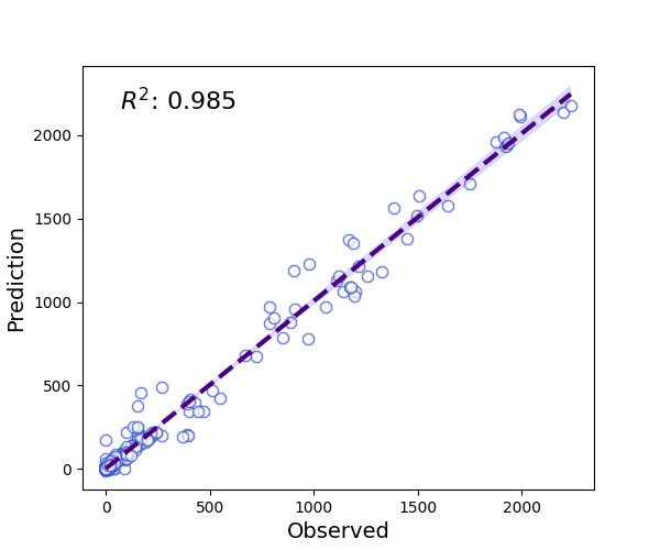
Test data
test_p = model.predict(x=X_test,)
argument test is deprecated and will be removed in future. Please
use 'predict_on_test_data' method instead.
evaluate_model(y_test, test_p)
mse 2205.2253237958316
rmse 46.95982670108389
r2 0.9851351044953288
r2_score 0.9847156482849592
mape inf
mae 20.746605740992923
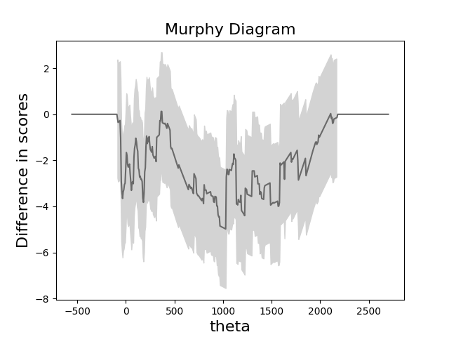
pp = ProcessPredictions(mode='regression', forecast_len=1, path=path)
pp.murphy_plot(y_test, test_p, prefix="test", where=path, inputs=X_test)
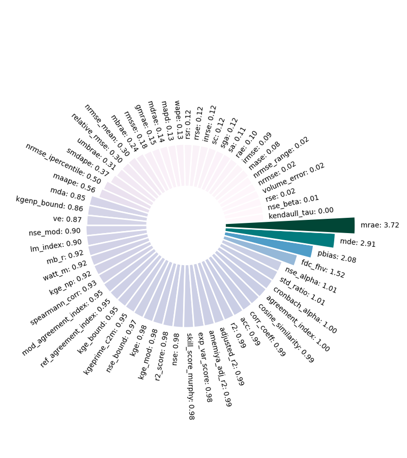
metrics = RegressionMetrics(y_test, test_p)
errors = metrics.calculate_all()

for err in ['kl_sym']:
    errors.pop(err)

n_errors = {}
for k,v in errors.items():
    if 0.<v<5.0:
        n_errors[k] = v

_ = circular_bar_plot(n_errors, sort=True, show=False, figsize=(8,9))
plt.tight_layout()
plt.show()
axes = regplot(pd.DataFrame(y_test), pd.DataFrame(test_p),
        marker_size=60,
        marker_color='snow',
        line_style='--',
        line_color='indigo',
        line_kws=dict(linewidth=3.0),
        scatter_kws=dict(linewidths=1.1, edgecolors=np.array([56, 86, 199])/255,
                         marker="8",
                         alpha=0.7
                         ),
        show=False
        )
axes.annotate(f'$R^2$: {round(RegressionMetrics(y_test,test_p).r2(), 3)}',
              xy=(0.3, 0.95),
              xycoords='axes fraction',
              horizontalalignment='right', verticalalignment='top',
              fontsize=16)
plt.show()
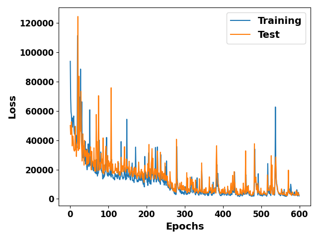
combined
legend_properties = {'weight':'bold',
                     'size': 14}

ax = plot(h.history['loss'], show=False, label='Training'
                    , ax_kws=dict(xlabel='Epochs', ylabel='Loss')
                    )
ax = plot(h.history['val_loss'], ax=ax, label='Test',
                show=False)

ax.set_ylabel(ylabel= 'Loss', fontsize=14, weight='bold')
ax.set_xlabel(xlabel='Epochs', fontsize=14, weight='bold')
ax.set_xticklabels(ax.get_xticks().astype(int), size=12, weight='bold')
ax.set_yticklabels(ax.get_yticks().astype(int), size=12, weight='bold')
ax.legend(prop=legend_properties)
plt.tight_layout()
plt.show()
FixedFormatter should only be used together with FixedLocator
FixedFormatter should only be used together with FixedLocator
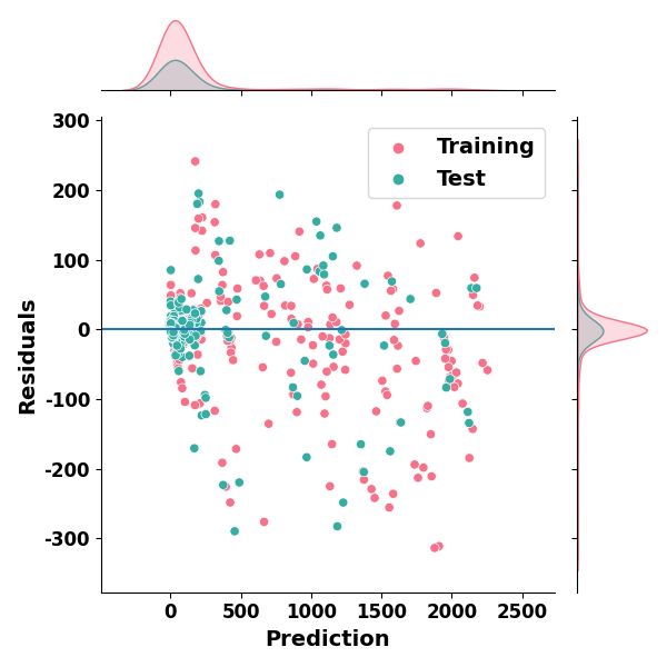
scatter plot of prediction and errors with KDE
train_er = pd.DataFrame((y_train - train_p), columns=['Error'])
train_er['prediction'] = train_p
train_er['hue'] = 'Training'
test_er = pd.DataFrame((y_test - test_p), columns=['Error'])
test_er['prediction'] = test_p
test_er['hue'] = 'Test'

df_er = pd.concat([train_er, test_er], axis=0)

legend_properties = {'weight':'bold',
                     'size': 14,}

g = sns.jointplot(data=df_er, x="prediction",
                     y="Error",
              hue='hue', palette='husl')
ax = g.ax_joint
ax.axhline(0.0)
ax.set_ylabel(ylabel= 'Residuals', fontsize=14, weight='bold')
ax.set_xlabel(xlabel='Prediction', fontsize=14, weight='bold')
ax.set_xticklabels(ax.get_xticks().astype(int), size=12, weight='bold')
ax.set_yticklabels(ax.get_yticks().astype(int), size=12, weight='bold')
ax.legend(prop=legend_properties)
plt.tight_layout()
plt.show()
FixedFormatter should only be used together with FixedLocator
FixedFormatter should only be used together with FixedLocator
legend_properties = {'weight':'bold',
                     'size': 14}
_, ax = plt.subplots(#figsize=(5,4)
                     )

edf_plot(np.abs(y_train-train_p), label='Training',
        c=np.array([200, 49, 40])/255,
         #c=np.array([234, 106, 41])/255,
         linewidth=2.5,
         show=False, ax=ax,)
edf_plot(np.abs(y_test-test_p),
         c=np.array([68, 178, 205])/255, linewidth=2.5,
         label='Test', ax=ax, show=False,
         ax_kws=dict(grid=True, xlabel='Absolute error'))
ax.set_ylabel(ylabel= 'Commulative Probabilty', fontsize=14, weight='bold')
ax.set_xlabel(xlabel='Absolute Error', fontsize=14, weight='bold')
ax.set_xticklabels(ax.get_xticks().astype(int), size=12, weight='bold')
ax.set_yticklabels(ax.get_yticks().round(2), size=12, weight='bold')
ax.legend(prop=legend_properties)
plt.title("Empirical Distribution Function Plot",fontweight="bold")
plt.tight_layout()
plt.show()

FixedFormatter should only be used together with FixedLocator
FixedFormatter should only be used together with FixedLocator
legend_properties = {'weight':'bold',
'size': 14}
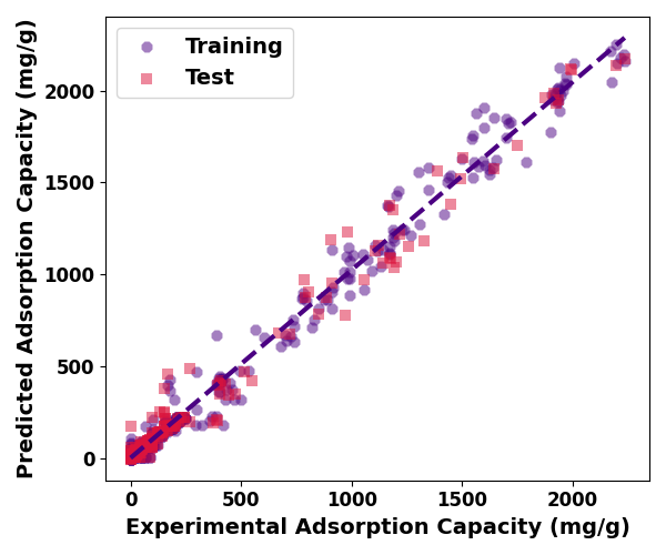
ax = regplot(pd.DataFrame(y_train), pd.DataFrame(train_p),
marker_size=60,
ci=False,
marker_color='indigo',
line_style='--',
line_color='indigo',
line_kws=dict(linewidth=3.0),
scatter_kws=dict(linewidths=0, edgecolors='snow',
marker="8",
alpha=0.5,
label='Training'
),
show=False
)
regplot(pd.DataFrame(y_test), pd.DataFrame(test_p),
marker_size=60,
ci=False,
marker_color='crimson',
line_kws=dict(linewidth=0),
scatter_kws=dict(linewidths=0, edgecolors='crimson',
marker="s",
alpha=0.5,
label='Test'
),
show=False,
ax=ax
)
ax.set_ylabel(ylabel= 'Predicted Adsorption Capacity (mg/g)', fontsize=14, weight='bold')
ax.set_xlabel(xlabel='Experimental Adsorption Capacity (mg/g)', fontsize=14, weight='bold')
ax.set_xticklabels(ax.get_xticks().astype(int), size=12, weight='bold')
ax.set_yticklabels(ax.get_yticks().astype(int), size=12, weight='bold')
ax.legend(prop=legend_properties)
plt.tight_layout()
plt.show()
FixedFormatter should only be used together with FixedLocator
FixedFormatter should only be used together with FixedLocator
legend_properties = {'weight':'bold',
'size': 14,}
fig, axes = plt.subplots(#figsize=(9,7)
)
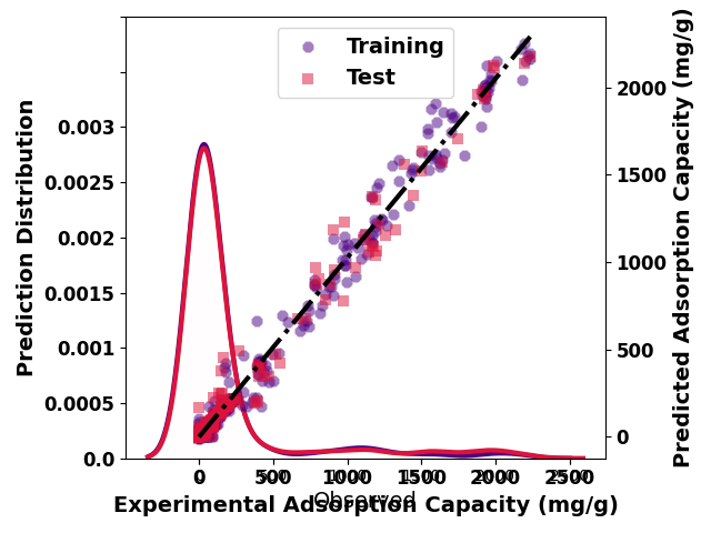
ax = ridge([train_p.reshape(-1,), test_p.reshape(-1,)],
color=['snow', 'snow'],
line_color=['indigo', 'crimson'],
line_width=3.0,
share_axes=True,
fill_kws={'alpha':0.05},
show=False,
ax=axes,
cut=0.15
)
ax[0].set_ylabel('Prediction Distribution', fontsize=14, weight='bold')
#ax[0].tick_params(axis='y', labelsize=15)
ax[0].set_xlabel('Experimental Adsorption Capacity (mg/g)', fontsize=14, weight='bold')
#ax[0].tick_params(axis='x', labelsize=15)
ax[0].set_xticklabels(ax[0].get_xticks().astype(int), size=12, weight='bold')
ax[0].set_yticklabels(ax[0].get_yticks(), size=12, weight='bold')
ax[0].set_ylim(-0, 0.004)
ax2 = ax[0].twinx()
ax2 = regplot(pd.DataFrame(y_train), pd.DataFrame(train_p),
marker_size=60,
ci=False,
marker_color='indigo',
line_style='-.',
line_color='black',
line_kws=dict(linewidth=3.0),
scatter_kws=dict(linewidths=0, edgecolors='snow',
marker="8",
alpha=0.5,
label='Training'
),
show=False,
ax=ax2,
)
ax2 = regplot(pd.DataFrame(y_test), pd.DataFrame(test_p),
marker_size=60,
ci=False,
marker_color='crimson',
line_kws=dict(linewidth=0),
scatter_kws=dict(linewidths=0, edgecolors='crimson',
marker="s",
alpha=0.5,
label='Test'
),
show=False,
ax=ax2
)
ax2.set_ylabel('Predicted Adsorption Capacity (mg/g)', fontsize=14, weight='bold')
ax2.set_yticklabels(ax2.get_yticks().astype(int), size=12, weight='bold')
ax2.legend(prop=legend_properties, loc = 'upper center')
plt.tight_layout()
plt.show()
FixedFormatter should only be used together with FixedLocator
FixedFormatter should only be used together with FixedLocator
FixedFormatter should only be used together with FixedLocator
scatter plot of true and predicted with train and test KDE
train_df = pd.DataFrame(np.column_stack([y_train, train_p]),
                        columns=['true', 'predicted'])

train_df['hue'] = 'Training'

test_df = pd.DataFrame(np.column_stack([y_test, test_p]),
                        columns=['true', 'predicted'])

test_df['hue'] = 'Test'

df = pd.concat([train_df, test_df], axis=0)

legend_properties = {'weight':'bold',
                     'size': 14,}

g = sns.jointplot(data=df, x="true",
                     y="predicted",
              hue='hue', palette='husl')

ax = g.ax_joint

ax.set_ylabel(ylabel= 'Predicted Adsorption Capacity (mg/g)', fontsize=14, weight='bold')
ax.set_xlabel(xlabel='Experimental Adsorption Capacity (mg/g)', fontsize=14, weight='bold')
ax.set_xticklabels(ax.get_xticks().astype(int), size=12, weight='bold')
ax.set_yticklabels(ax.get_yticks().astype(int), size=12, weight='bold')
ax.legend(prop=legend_properties)
plt.tight_layout()
plt.show()

FixedFormatter should only be used together with FixedLocator
FixedFormatter should only be used together with FixedLocator
Total running time of the script: (0 minutes 51.794 seconds)